Verbatim coding and sample size
July 31, 2018
Coding verbatims into concepts is a common task in text analytics. But how many concepts should you expect to find given your sample size? How big should your sample be to identify 20 concepts?
That may sound abstract, but when budgeting research that's the bet we make with actual dollars. It'd be good to know the odds.
This article suggests a new way to predict how many distinct codes you may expect to see in N survey responses. Such a curve might be used to inform sample size selection before fielding research, or during analysis to benchmark the results.
Background
Text verbatims are awesome as they're one of the few ways your survey can tell you something you didn't already know. But how many respondents do you need to recruit to be confident you'll learn something new?
The more responses you get, the more likely you are to see new ideas. But the more responses you get, the more likely it is that the next response is similar to something you've seen before.
Case study
A survey asked 200 patients why they liked a particular medical device.
The response returned a wide array of responses.
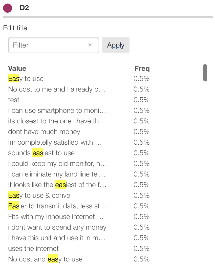
Scanning the data suggests concepts that might be the basis for coding.
Here a number of answers suggest the idea of "Easy" highlighted in yellow:

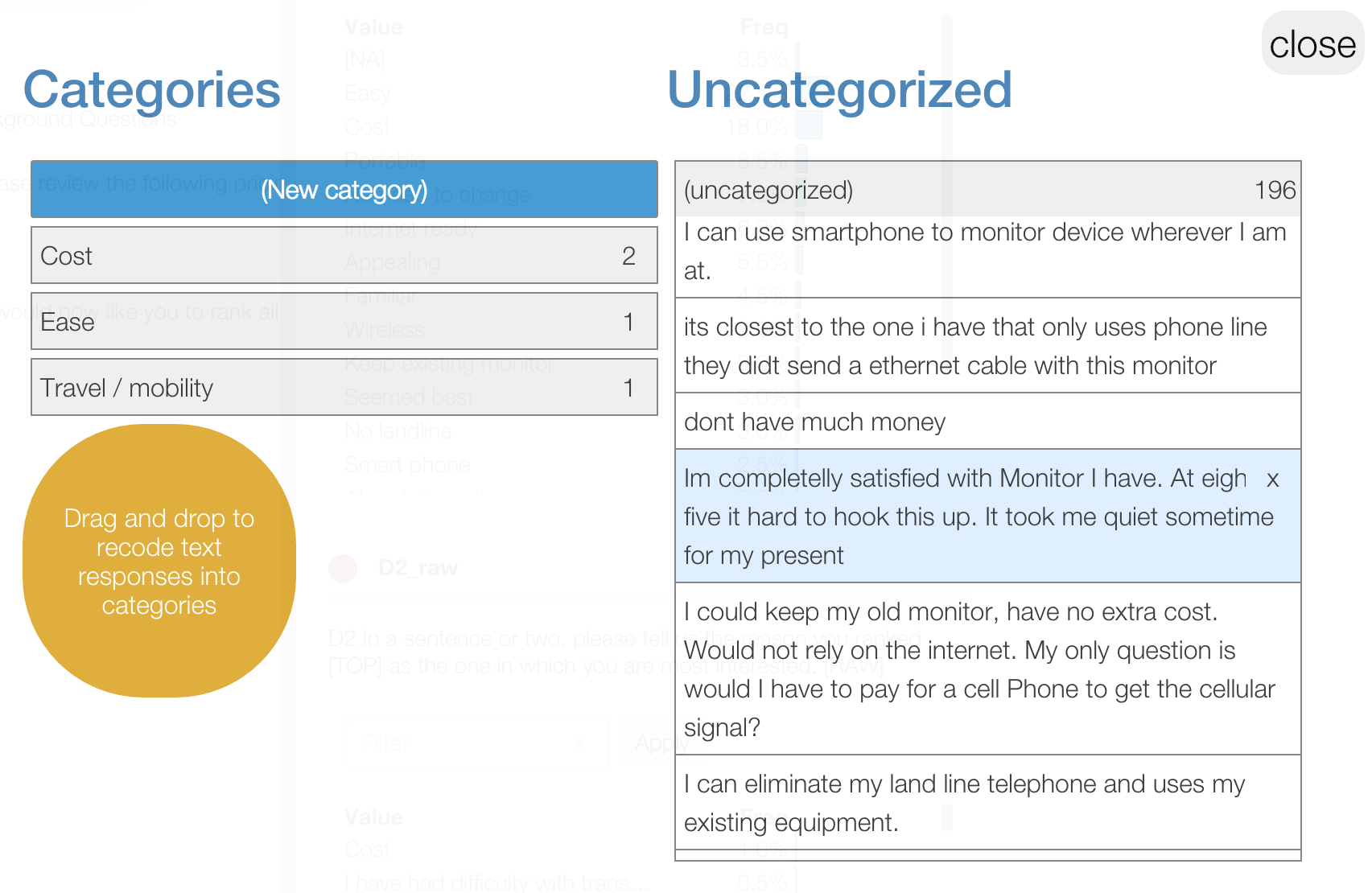
Protobi provides a few tools for coding text verbatims, described in this tutorial Advanced recoding tool

In this project, the client coded raw verbatim text responses from each respondent into categories. Some responses included compound answers that were coded to more than one concept, e.g. "Affordable and easy to use".
Below is a chart showing the count of responses behind each code. The most common codes were "Easy" (n=44), "Cost" (n=36) and "Portable" (n=18).
Zipf's Law
We can see here the distribution has a "long tail" with a few high-frequency codes and many low-frequency ones.
According to Zipf's Law we'd expect the frequency of each code to be inversely proportional to its rank:
Zipf's law can be derived from the power-law probability distribution, which describes many long-tail phenomena.
In the graph above, the actual frequencies are plotted as dots. The two lines show a slope of -1 (α=1) for reference.
Heap's Law
If the frequency of codes follows Zipf's Law, then the cumulative number of distinct codes we'd expect to encounter at any given sample size is described by Heap's Law:
where N(t) is the number of distinct codes we would expect to find in t responses, and k and β are estimated empirically.
And in the special case where α=1 in the Zipf distribution, then there is an exact formula for Heap's Law based on the Lambert W function:
Lambert's W function
It's striking that the W function should appear here, as we've recently seen it arise in a very different context Optimal Price in Descrete Choice Models and was only identified as a named as recently as 1993 by Donald Knuth et al (see "On Lambert's W Function").
So what?
The most common codes are already likely to be unsurprising. In this case, the client already anticipated "Cost", "Ease" and "Uses cell phone" based on prior market knowledge. It's the codes that emerge with more data that yield new insights.
After a number of responses were coded, the client created different code related to the cell phone:
- "Uses cell phone - can drop landline"
- "Uses cell phone - I can travel now"
- "Uses cell phone - I don't need to buy a new device"
These distinctions provided new insights into the marketing strategy, and started to become apparent after they had coded 100-150 responses.
Summary
Of course it's not possible to predict exactly how many verbatim codes you'll end up with . But it's safe to say that
- the more responses you collect, the more concepts you can identify,
- the rate at which you identify new codes will decrease.
This article provides empirical curves based on other research domains that may help predict how many concepts we might expect to find based on the sample size.
