Estimate and profile segmentations
September 3, 2014
Here's how to to compute candidate market segmentations using R and profile them in Protobi, using the most recent StackOverflow Developer Survey as a case study.
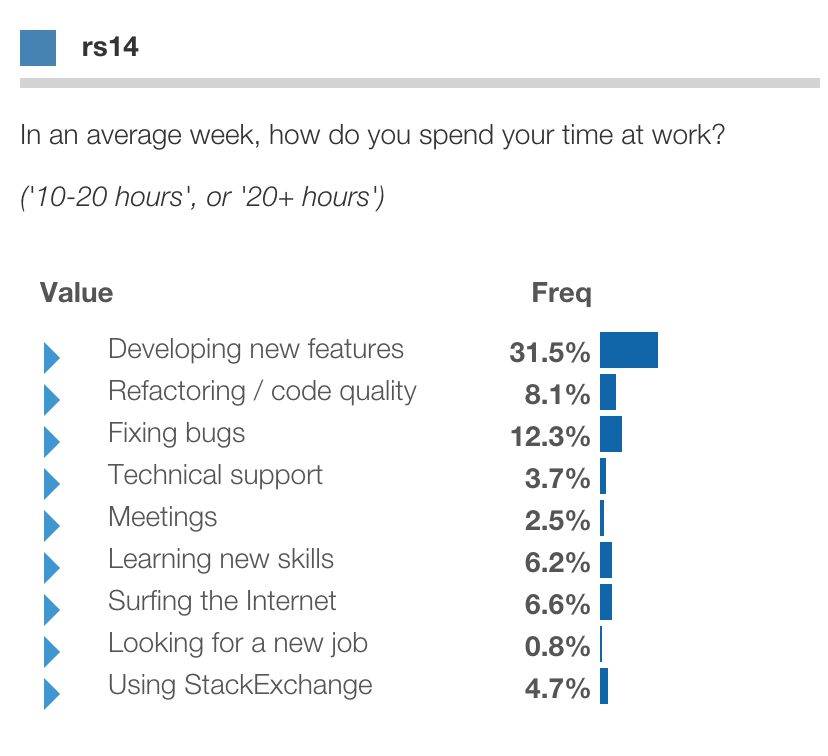
This yields a simple segmentation of developers based on what tasks they spend their time on ( note how little time in any country spent looking for a new job...)
Overview
There are many good ways to develop candidate segmentations, including K-means clustering, CART/CHAID, and even sheer business insight. Different analysts can reasonably differ on the best algorithm to use for a given task, or even take multiple approaches using Random Forests.
But whatever algorithm(s) used, almost every segmentation analysis will generate multiple alternative segmentations. Additionally, it's common practice to give each segment a mnemonic name.
But how do you evaluate and choose among the candidates? How do you get a qualitative sense of each segment, to choose a name?
We argue here that a good first step is to simply look at it. and show how using Protobi.
The goal here is not to show the only way to go about it, but to show one practical workflow.
StackOverflow Survey
StackOverflow conducted a survey of its members. Click here to explore the data in Protobi.
One of the questions was "In an average week, how do you spend your time at work?" for an array of tasks, such as "New feature development", "Meetings", or "Looking for a new job".
Respondents selected a single choice of "None", "1-2 hours", "2-5 hours", "5-10 hours", "10 to 20 hours", or "20+ hours". The above graph shows percent of respondents who selected "10 to 20 hours" or "20+ hours" for each task.
This example develops a segmentation based on responses to this section.
Latent Class Segmentation in R
Here we use Latent Class Analysis using the poLCA library in R to derive candidate segmentations, and attach predicted segment membership back to the original datafile for evaluation. (An analogous process can be done using LatentGold, QUICK CLUSTER in SPSS or FASTCLUS in SAS.)
The basic steps are:
- Import data
- Recode basis variables
- Segment respondents into various numbers of clusters
- Marge back predicted segment membership
- Export data
Step 1: Load the relevant packages and read the input dataset. You can find the data here in SAV format at 2013_StackOverflowRecoded.sav and 2013_StackOverflowRecoded.csv.
Step 2: A quirk of poLCA is that the variables used as the segmentation basis must be coded as a sequence
of integers starting with 1 (i.e. 1, 2, 3, ...). Here the values are already coded as a sequence of integers,
but starting at 0, so we increment them by 1 using the recode method in the car library.
Step 3: Run cluster analyses to create solutions with 2-, 3-, 4-, 5- and 6-clusters, respectively.
The poLCA algorithm treats all basis variables as categorical, not ordinal or continuous.
There's an inherent ordinality in our coding, which it thus can't recognize whereas the more sophisticated algorithms in
LatentGold from Statistical Innovations can.
Note that we set na.rm=TRUE which means that respondents with missing values
will be included, and NA treated as its own category.
Step 4: Finally, we merge the predicted class memberships from each solution back to the main data frame
Step 5: Export as a new CSV file. That's the data we'll view in Protobi.
The complete R program is below:
# Step 1:  Load packages,  libraries and data
install.packages("car");
install.packages("poLCA");
install.packages("scatterplot3d");  # required by poLCA
install.packages("MASS"); # required by poLCA
library(car); # for recoding
library(poLCA); # for segmentation

so <- read.csv("2013_StackOverflowRecoded.csv", header=TRUE, sep=",")
Step 2: Recode basis variables to positive integers starting at one
so$rs14_1 <- recode(so$q14_1,"5=6;4=5;3=4;2=3;1=2;0=1;")
so$rs14_2 <- recode(so$q14_2,"5=6;4=5;3=4;2=3;1=2;0=1;")
so$rs14_3 <- recode(so$q14_3,"5=6;4=5;3=4;2=3;1=2;0=1;")
so$rs14_4 <- recode(so$q14_4,"5=6;4=5;3=4;2=3;1=2;0=1;")
so$rs14_5 <- recode(so$q14_5,"5=6;4=5;3=4;2=3;1=2;0=1;")
so$rs14_6 <- recode(so$q14_6,"5=6;4=5;3=4;2=3;1=2;0=1;")
so$rs14_7 <- recode(so$q14_7,"5=6;4=5;3=4;2=3;1=2;0=1;")
so$rs14_8 <- recode(so$q14_8,"5=6;4=5;3=4;2=3;1=2;0=1;")
so$rs14_9 <- recode(so$q14_9,"5=6;4=5;3=4;2=3;1=2;0=1;")
Step 3: Compute segmentation using above columns as the segmentation basis
q14rs <- cbind(rs14_1, rs14_2, rs14_3, rs14_4, rs14_5, rs14_6, rs14_7, rs14_8, rs14_9) ~ 1
q14clu2 <- poLCA(q14rs, so, nclass=2, na.rm=FALSE); # BIC(2): 163650.3
q14clu3 <- poLCA(q14rs, so, nclass=3, na.rm=FALSE); # BIC(3): 161445.0
q14clu4 <- poLCA(q14rs, so, nclass=4, na.rm=FALSE); # BIC(4): 160172.9
q14clu5 <- poLCA(q14rs, so, nclass=5, na.rm=FALSE); # BIC(5): 159428.3
q14clu6 <- poLCA(q14rs, so, nclass=6, na.rm=FALSE); # BIC(6): 159209.8
Step 4: merge estimated segment membership back to main data frame
so$q14_clu2 <- q14clu2$predclass
so$q14_clu3 <- q14clu3$predclass
so$q14_clu4 <- q14clu4$predclass
so$q14_clu5 <- q14clu5$predclass
so$q14_clu6 <- q14clu6$predclass
Step 5: export augmented data as a new CSV
write.table(so, file="2013_StackOverflowRecoded_lca.csv", sep=",", col.names=TRUE,qmethod="double", na="", row.names=FALSE)
Visualize segments in Protobi
We had first created a project based on the original dataset, and organized that view nicely. So we updated the project in-place with the new augmented dataset. This allows us to keep the same map but add/drop fields with possibly new records or field values.
There are several new fields, corresponding to each cluster solution, including the 3-cluster solution, q14clu_3.
At first it's unnamed, with just the values 1, 2 and 3. We can get a sense of their character by drilling into each
value and looking for significant differences.
Candidate segment 1
For instance, below we click into value q14clu_3 = 1:
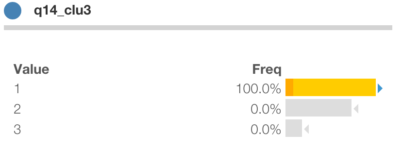
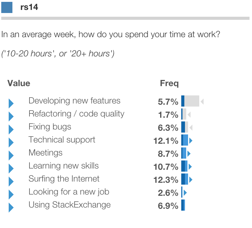
Here the values for respondents in this segment are shown in blue. The baseline distribution for all respondents is shown as a light grey shadow for comparison.
We can see that Segment 1 is significantly less likely (as indicated by the gray arrow icon)
to spend a lot of time on new features or refactoring,
and a lot more time on meetings, technical support, new skills and everything else. We might call these "All but dev".
Candidate segment 2
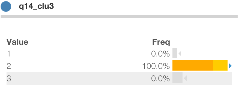
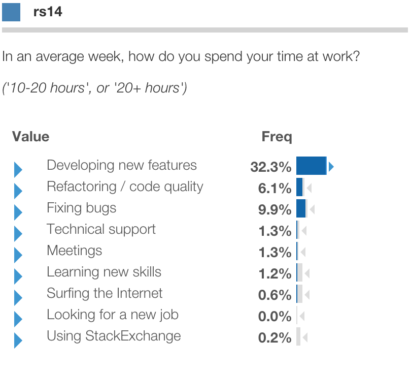
Below is segment 2. These respondents are quite the opposite, focused almost exclusively on new features and code quality:
Candidate segment 3
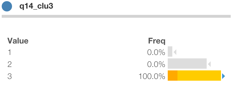
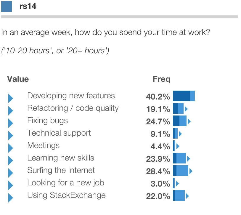
Finally is segment 3. These respondents are even more likely than Segment 2 to spend a lot of time on new features and quality,
yet even more likely than segment 1 to spend a lot of time in meetings, tech support and learning new skills.
We might call this segment "Dev and growth" (to be literal) or perhaps "Entrepreneur" (to apply a bit of descriptive license).
Profile a segmentation
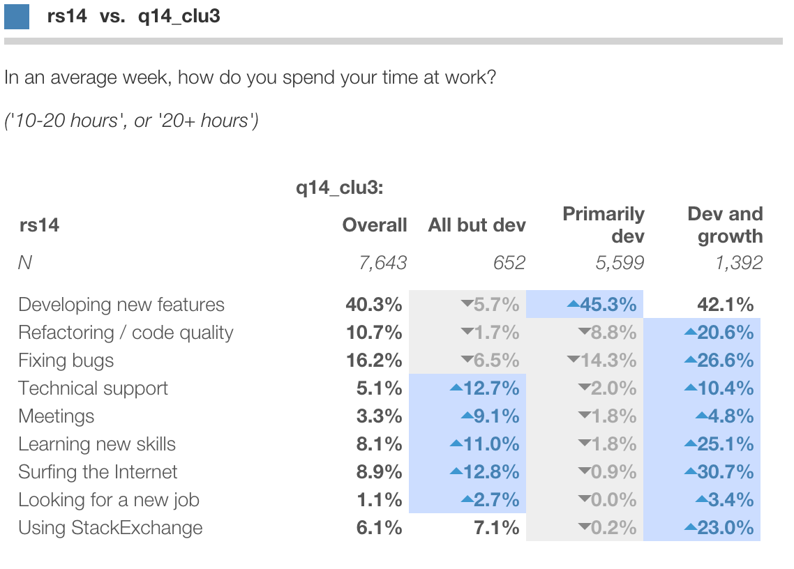
So now we can name the segments:
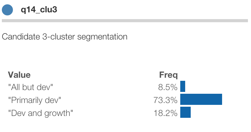
Clicking and contrasting is fun and informative for exploratory analysis. But to present it to the client, we might aim for a more concise crosstab (which we can copy to Excel and create a stylized custom chart):
Compare alternative segmentations
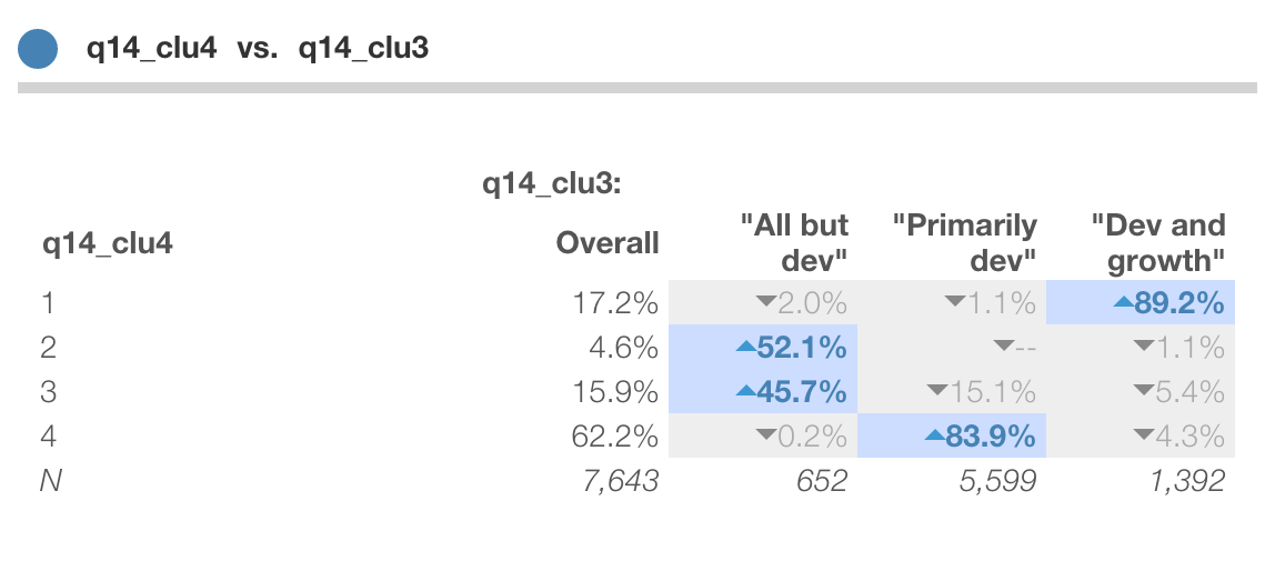
Wait ... what about the four-cluster solution? How's that different? Might that be better? Let's take a look!
One thing we can do is crosstab two candidate solutions. That's easy to do in Protobi by dragging the header of one to the header of the other.
For instance, we can compare the 4-cluster solution to the 3-cluster solution. Here we can see that
- segment
4-1corresponds to3-3("Dev and growth") - segment
4-4corresponds to3-2("Primarily dev"). - segments
4-2and4-3split3-1("All but dev.")
This post provides a brief tutorial on how to estimate candidate segmentations in an external software package, and visualize the resulting segmentations in Protobi.
Summary
Try Protobi with your next segmentation project, and let our expert analysts show you how.
